Moving Averages and Statistics for Stock Prices

1. Finding Historical Prices

import requests

In site url, period1 is starting time, period 2 is ending time

site="https://query1.finance.yahoo.com/v7/finance/download/2330.TW?period1=0&period2=1549258857&interval=1d&events=history&crumb=hP2rOschxO0"
response = requests.post(site)

Now historical data of 2330.TW is stored in "response". To check text file:

print(response.text)

To save file as csv

with open('file.csv', 'w') as f:
f.writelines(response.text)
print(df.head())

To improve csv file

• parse_dates changes first column to datetime (instead of 0,1,2,3)

import pandas as pd
df = pd.read_csv('file.csv', index_col='Date', parse_dates=['Date'])
print(df.head())

import numpy as np
import pandas as pd
import pandas_datareader as pdr
import matplotlib.pyplot as plt
%matplotlib inline

Dataframe setting 2019-04-17 as starting date

gld = pdr.get_data_yahoo('GLD', '2019-04-17')
gld.head()

 

Compute moving averages

gld_close = pd.DataFrame(gld.Close)

gld_close['MA_9'] = gld_close.Close.rolling(9).mean().shift()
gld_close['MA_21'] = gld_close.Close.rolling(21, center=True).mean() 

Make sure data doesn't have gaps

gld_close['MA_9'].head(12)

Plotting 9 days and 21 days average of gold prices

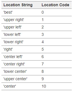
• legend(loc='upper right', shadow=True) determines position of label

plt.figure(figsize=(15,10))
plt.grid(True)
plt.plot(gld_close['Close'], label='GLD')
plt.plot(gld_close['MA_9'], label = 'MA 9 day')
plt.plot(gld_close['MA_21'], label = 'MA 21 day')
plt.legend(loc=2)

Computate historical volatility in options

• Close divided by previous days close

gld_close["change"] = np.log(gld_close["Close"] / gld_close["Close"].shift())

plt.plot(gld_close.change)

 

Compute using rolling standard deviation., 21 day method

• Average trading days each month is 21
• 21 observations, use volatility from the next day so shift by 1
• Cleaner version of former graph

gld_close['Volatility'] = gld_close.change.rolling(21).std().shift()
gld_close['Volatility'].plot()

• Tips: Special arrows and words: ax.annotate(s="second node", xy=(8,1), xytext=(5,1.5), arrowprops=dict(arrowstyle='->', connectionstyle="arc3, rad=.2"))
• Subplot: fig, ax = plt.subplots()
• axe_base = plt.axes()
• axe_small = plt.axes([0.65, 0.65, 0.2, 0.2]) ----> ([bottom, left, width, height])

2. Basic Stock Price Analysis

Add column expected change as "exp_chng". Closing price multiplied by 1 standard deviation (=21 day rolling sd). Use volatility to predict 1 sd move tomorrow

Add another column actual change as "gld_close". Closing price yesterday minus today

gld_close['exp_chng'] = gld_close['Volatility'] * gld_close['Close'].shift()
gld_close['actual_chng'] = gld_close['Close'] - gld_close['Close'].shift()
gld_close.head()

 

Slice off rows with NaN data

gld_close = pd.DataFrame(gld_close.iloc[22:])

Magnitude of change

• Actual change/ Expected change. Make column in standard deviations

gld_close['Magnitude'] = gld_close['actual_chng'] / gld_close['exp_chng']

Plot Histogram

• Bins arguments add more columns. Defaults around 10
• Plot against standard deviation
• Likely in negative change than positive side

plt.hist(gld_close['Magnitude'], bins=50)

Scatter Plot

Add absolute magitude column

gld_close['abs_magni'] = np.abs(gld_close['Magnitude']

Shows price changes

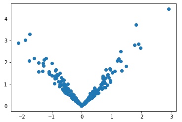
• x axis in dollars, y axis absolute value in s.d.
• Most around 2.5 s.d. movement

plt.scatter(gld_close['actual_chng'], gld_close['abs_magni'])

3. Correlation Matrix 

pip install fix-yahoo-finance

pip install pandas-datareader

Setup environment

import numpy as np
import pandas as pd
import fix_yahoo_finance as fyf

 Download data for FANG stocks

• Store downloaded data as "data"
• Automatically sorted name alphabetically

stocks = 'FB AMZN NFLX GOOG AAPL'
stocks = stocks.split()
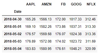
data = fyf.download(stocks, '2018-05-01')['Close']
data.head()

import matplotlib.pyplot as plt
%matplotlib inline
plt.plot(data)
plt.legend(['AMZN', 'FB', 'GOOG', 'AAPL', 'NFLX'], loc=2)

Transform closing price to rates of return

• Store instanteous data in dataframe called "returns"
• Loop through securities download, ensure not duplicated data

returns = pd.DataFrame()
for stock in data:
if stock not in returns:
returns[stock] = np.log(data[stock]).diff()
returns = returns[1:]
returns.head()

Shows average, min, max, std, 25% etc.

returns.describe()

Shows correlation table

returns.corr()

Display correlation to AMZN in descending order of correlation

returns.corr()['AMZN'].sort_values(ascending=False)

AMZN 1.000000
GOOG 0.768602
NFLX 0.705024
AAPL 0.674327
FB 0.578970
Name: AMZN, dtype: float64

Shows scatter matrix

from pandas.plotting import scatter_matrix
scatter_matrix(returns, figsize=(16,12), alpha=0.3)